Flagging is a way of identifying records for which there is a strong likelihood that values of anthropometric measurements or the age of the child are incorrect. Records can then be checked and corrected, or censored (i.e. excluded) from subsequent analyses.
Flagging is a process of checking whether values of anthropometric indices are outside a given range and recording the result in one or more new variables. The result may be a set of logical (i.e. 1/0 or true/false) flag variables (i.e. one flag variable per anthropometric index) or a single variable holding a code number that classifies the nature of the detected problem(s).
Flagging is usually applied to height-for-age z-scores (HAZ), weight-for-age z-scores (WAZ), weight-for-height z-scores (WHZ), and BMI-for-age z-scores (BAZ) calculated from data collected during nutritional anthropometry surveys. The flagging process can be easily applied to other variables.
Two flagging criteria for anthropometric indices are in common use internationally. These are the WHO flagging criteria and the SMART flagging criteria. Both methods flag records in which one or more anthropometric indices are more than a certain distance either side of a reference value. The two methods are summarised in table below.
| Lower limit | Upper limit | Lower limit | Upper limit | Lower limit | Upper limit | Lower limit | Upper limit | Reference value | |
|---|---|---|---|---|---|---|---|---|---|
| WHO | -6 | +6 | -6 | +5 | -5 | +5 | -5 | +5 | Zero |
| SMART | -3 | +3 | -3 | +3 | -3 | +3 | NA | NA | Survey sample |
| 1 Indices are height-for-age z-score (HAZ), weight-for-age z-score (WAZ), weight-for-height z-score (WHZ), and BMI-for-age z-score (BAZ). | |||||||||
| 2 NA = Not available. BAZ is not used in SMART surveys. SMART flagging criteria for BAZ are undefined. |
Applying flagging criteria is a matter of checking that individual values of these indices are within the lower and upper limits shown in the table above. Values that are outside of these limits are flagged in a new variable.
The WHO criteria are simple biologically plausible ranges. If, for example, a value for WHZ is below -5 or above +5 then the record is flagged to indicate a likely problem with WHZ. This will usually be caused by an erroneous weight or height value being recorded.
Note that values outside of these flagging limits may be observed in children admitted into (e.g.) therapeutic feeding programs.
SMART criteria are more complicated. They require the mean value of the index to be calculated from the survey data. This is then used as the reference value. For example, if a value for WHZ is below:
or above:
then the record is flagged to indicate a likely problem with WHZ.
A mean WHZ of -1.15 gives lower and upper SMART flagging limits of:
and:
respectively. These limits may incorrectly flag biologically plausible values. See figure below.
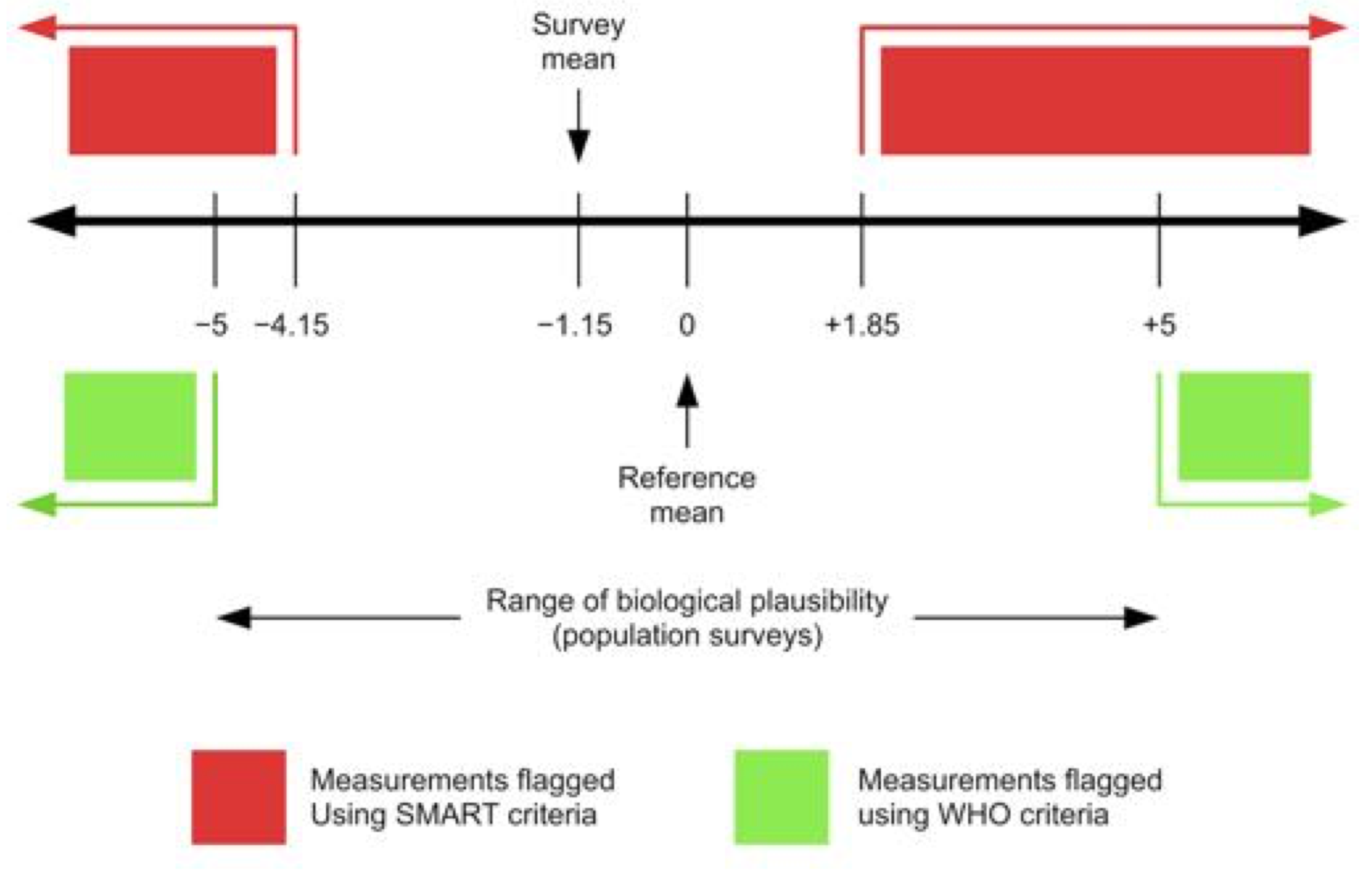
Example of WHO and SMART flagging criteria for weight-for-height z-scores (WHZ)
The WHO and SMART flagging criteria will flag different but overlapping sets of measurements. This means that survey results can be affected by the flagging criteria used. This is because the prevalence of an indicator describes the proportion of values in one of the “tails” of the distribution of an index (see figure below).
The SMART flagging criteria will usually flag more records than the WHO flagging criteria. This will act to reduce estimated prevalence (see figure below). This will be a particular problem when the prevalence of severe forms of undernutrition is high.
There are some problems with using the SMART flagging criteria:
Flagging is about detecting outlier values. The SMART flagging criteria use distance from the sample mean, but the value of the mean can be strongly influenced by the presence of outliers. This could be overcome by, for example, using the median or a trimmed mean as the reference mean. If you do this you will not be using the SMART flagging criteria.
SMART flagging criteria are supposed to define outliers using statistically plausible limits. The underlying principle is that, for a normally distributed variable, we expect 99.87% of all values to lie within three sample standard deviations of the sample mean. If we exclude records with values more than three standard deviations from the mean then we would incorrectly flag very few records (i.e. 0.13% of the total) as problematic. The SMART method assumes that the distribution of each anthropometric index in a population is always perfectly normal and that the standard deviation is always exactly one. This assumption is almost always violated. If it is violated then the use of the SMART flagging criteria may lead to records being flagged inappropriately. There are ways (e.g. transforming data toward normality, using the sample standard deviation) to avoid this problem but using them would also not be using the SMART flagging criteria.
Wide-area surveys such as MICS and DHS will usually collect data from many populations. Each population may have different distributions of anthropometric indices and different prevalence of anthropometric indicators. In this case the mean of the entire survey sample will not be a suitable reference mean and the assumed standard deviation (i.e. SD = 1) will usually be too narrow to set limits that define statistical outliers. This will lead to records being flagged incorrectly. This is illustrated in Figure F3. Stratum or district specific means should be used instead of whole sample means, but this may not solve the problem entirely.
If SMART flagging criteria have already been applied to data and the flagged records have been removed from the dataset then a subsequent application of the SMART flagging criteria will tend to flag additional records. SMART flagging criteria should, therefore, only be applied to raw data. Do not apply SMART flagging criteria to data from which flagged records have been removed.
It is important to note that only one set of flagging criteria, either WHO or SMART, should be used at any one time.
The WHO and SMART flagging criteria are designed to be applied to survey samples. They should not be applied to clinical populations or samples.
Software such as ENA from SMART, EpiInfo, WHO Anthro, WHO AnthroPlus, and scripts / macros for R, SAS, SPSS, and STATA provided by the WHO are frequently used to calculate anthropometric indices and apply flagging criteria to data from surveys that collect anthropometric data. It is quite common to receive data to which flagging criteria have already been applied and contain one or more flag variables. You may use these flags if you are sure which flagging criteria have been applied. If you are unsure which flagging criteria have been applied then you should apply your flagging criteria of choice using one of these software packages or the procedures outlined in this section. You may also need to recalculate anthropometric indices using WHO reference values if they were calculated using NCHS, CDC, or local growth references.
Applying WHO flagging criteria to survey data
For a first exercise, we will apply the WHO flagging criteria to survey data.
We will retrieve a survey dataset:
svy <- read.table("flag.ex01.csv", header = TRUE, sep = ",")#> psu child age sex weight height muac oedema haz waz whz
#> 1 1 1 20 2 6.1 82.5 127 2 -0.07 -4.54 -6.03
#> 2 1 2 13 2 6.4 70.4 116 2 -1.83 -3.04 -2.93
#> 3 1 3 15 1 7.1 67.5 124 2 -4.60 -3.34 -1.25
#> 4 1 4 15 1 7.2 75.4 130 2 -1.48 -3.22 -3.57
#> 5 1 5 15 1 7.4 70.0 124 2 -3.61 -2.99 -1.61
#> 6 1 6 18 2 7.7 70.6 130 2 -3.48 -2.40 -0.82The file flag.ex01.csv is a comma-separated-value (CSV) file containing anthropometric data from a recent SMART survey in Sudan.
Applying WHO flagging criteria is straightforward. We first create a column that will contain the flag code and set this to zero (i.e. no flags) for all records:
svy$flag <- 0#> psu child age sex weight height muac oedema haz waz whz flag
#> 1 1 1 20 2 6.1 82.5 127 2 -0.07 -4.54 -6.03 0
#> 2 1 2 13 2 6.4 70.4 116 2 -1.83 -3.04 -2.93 0
#> 3 1 3 15 1 7.1 67.5 124 2 -4.60 -3.34 -1.25 0
#> 4 1 4 15 1 7.2 75.4 130 2 -1.48 -3.22 -3.57 0
#> 5 1 5 15 1 7.4 70.0 124 2 -3.61 -2.99 -1.61 0
#> 6 1 6 18 2 7.7 70.6 130 2 -3.48 -2.40 -0.82 0Then we apply the flagging criteria for each index. Here we apply the WHO flagging criteria to the HAZ index:
#>   psu child age sex weight height muac oedema   haz   waz   whz flag
#> 1   1     1  20   2    6.1   82.5  127      2 -0.07 -4.54 -6.03    0
#> 2   1     2  13   2    6.4   70.4  116      2 -1.83 -3.04 -2.93    0
#> 3   1     3  15   1    7.1   67.5  124      2 -4.60 -3.34 -1.25    0
#> 4   1     4  15   1    7.2   75.4  130      2 -1.48 -3.22 -3.57    0
#> 5   1     5  15   1    7.4   70.0  124      2 -3.61 -2.99 -1.61    0
#> 6 1 6 18 2 7.7 70.6 130 2 -3.48 -2.40 -0.82 0This can be translated as “if HAZ is not missing and HAZ is below -6 or HAZ is above +6 then add 1 to the flag variable else leave the flag variable unchanged”.
Be careful when using the comparison operator with negative numbers. Always insert a space between the and characters. R interprets as an assignment operator and may produce unexpected and unwanted results without issuing a warning or error message.
Here we apply the WHO flagging criteria to the WHZ index:
#>   psu child age sex weight height muac oedema   haz   waz   whz flag
#> 1   1     1  20   2    6.1   82.5  127      2 -0.07 -4.54 -6.03    2
#> 2   1     2  13   2    6.4   70.4  116      2 -1.83 -3.04 -2.93    0
#> 3   1     3  15   1    7.1   67.5  124      2 -4.60 -3.34 -1.25    0
#> 4   1     4  15   1    7.2   75.4  130      2 -1.48 -3.22 -3.57    0
#> 5   1     5  15   1    7.4   70.0  124      2 -3.61 -2.99 -1.61    0
#> 6   1     6  18   2    7.7   70.6  130      2 -3.48 -2.40 -0.82    0
Here we apply the WHO flagging criteria to the WAZ index:
#>   psu child age sex weight height muac oedema   haz   waz   whz flag
#> 1   1     1  20   2    6.1   82.5  127      2 -0.07 -4.54 -6.03    2
#> 2   1     2  13   2    6.4   70.4  116      2 -1.83 -3.04 -2.93    0
#> 3   1     3  15   1    7.1   67.5  124      2 -4.60 -3.34 -1.25    0
#> 4   1     4  15   1    7.2   75.4  130      2 -1.48 -3.22 -3.57    0
#> 5   1     5  15   1    7.4   70.0  124      2 -3.61 -2.99 -1.61    0
#> 6   1     6  18   2    7.7   70.6  130      2 -3.48 -2.40 -0.82    0
Note that each time we apply a flagging criteria we increase the value of the flagging variable by the next power of two when a problem is detected:
We started with zero

Then we added $2 ^ 0$ (i.e. 1) if HAZ was out of range.

Then we added $2 ^ 1$ (i.e. 2) if WHZ was out of range.

Then we added $2 ^ 2$ (i.e. 4) if WAZ was out of range.
If we had another index then we would use (i.e. 8) to flag a problem in that index.
The advantage of using this coding scheme is that it compactly codes all possible combinations of problems in a single variable (see table below).
There are a number of flagged records in the example dataset. This:
table(svy$flag)returns:
#>
#>   0   1   2   3   5   6
#> 751   9  12   9   2   3
This table shows the relative frequency of detected problems. See table below to find the meaning of each of the codes.
| Code | HAZ | WHZ | WAZ | Suggested action(s) |
|---|---|---|---|---|
| 0 | O | O | O | None |
| 1 | X | O | O | Check height and age |
| 2 | O | X | O | Check weight and height |
| 3 | X | X | O | Check height |
| 4 | O | O | X | Check weight and age |
| 5 | X | O | X | Check age |
| 6 | O | X | X | Check weight |
| 7 | X | X | X | Check age, height, and weight |
The number of flagged records can be found using:
table(svy$flag != 0)["TRUE"]which returns:
#> TRUE
#>   35
The proportion of records that are flagged can be found using:
prop.table(table(svy$flag != 0))["TRUE"]This returns:
#>       TRUE
#> 0.04452926
About 4.45% of records are flagged.
Note that missing values are not flagged. It can be useful to check missing values to see if there are missing component measurements or if a component measurement is out of range for the calculation of index values (e.g. WAZ is only calculated for children aged ten years or younger). This issue can be explored by selection and listing. For example:
This returns:
#>   weight height whz
#> 8    8.1     NA  NA
There is one missing value for whz in record 8.This is due to a missing value for height (shown as NA). and haz will also be missing. It may be possible to fix this issue if the missing data are available on paper forms.
Flagging has a dual role:
It is a data-checking tool. If you have access to data collection forms you will be often able to check records and fix data-entry errors in the data.
It is a measure of data-quality. Flagged records can indicate problems with measurement, recording, data-entry, and data-checking. The proportion of flagged records in a dataset should, ideally, be below about 2.5%. SMART guidelines consider proportions above 7.5% to be problematic. We found that 4.45% of records in the example dataset were flagged. The data are of acceptable quality.
We can use:
svy[svy$flag != 0, ]
#>     psu child age sex weight height muac oedema   haz   waz   whz flag
#> 1     1     1  20   2    6.1   82.5  127      2 -0.07 -4.54 -6.03    2
#> 29    1    29  24   2   16.3  107.3  155      2  6.69  2.69 -0.82    1
#> 32    2     1  12   1    6.1   99.4  112      2  9.95 -4.02 -9.18    3
#> 35    2     4  24   2    6.8   65.5  128      2 -6.27 -4.30 -0.63    1
#> 88    3    30  24   2   16.9  107.5  158      2  6.75  2.95 -0.47    1
#> 106   4    18  36   1   13.4   65.7  152      2 -8.20 -0.56  7.64    3
#> 174   7     3  36   2    6.8   66.6  134      2 -7.47 -5.35 -1.01    1
#> 198   8     1  27   2    5.5   66.0  112      2 -6.59 -5.92 -3.27    1
#> 280  11     7  24   1    6.7   81.7  140      2 -1.77 -4.86 -5.63    2
#> 286  11    13  48   1    9.4   77.3  146      2 -6.21 -4.25 -0.69    1
#> 292  11    19  12   1   12.9   92.3  152      2  6.97  2.68 -0.50    1
#> 307  12     3  36   1    7.5   90.0  130      2 -1.64 -4.99 -6.42    2
#> 350  14     1  20   1    5.7   77.8  142      2 -2.27 -5.49 -6.47    2
#> 352  14     3  48   1    6.5   80.7  140      2 -5.40 -6.22 -5.74    6
#> 368  14    19  48   1   13.4   66.3  144      2 -8.83 -1.58  7.33    3
#> 399  15    21  36   1   14.3   66.0  154      2 -8.12 -0.02  8.58    3
#> 400  15    22  48   1   14.5   68.0  152      2 -8.42 -0.95  7.80    3
#> 405  16     4  24   2    7.8   65.0  145      2 -6.42 -3.27  1.04    1
#> 406  16     5  12   1    7.8   98.0  138      2  9.36 -1.93 -7.23    3
#> 408  16     7  48   1    8.0   77.0  128      2 -6.28 -5.20 -2.66    1
#> 432  17     3   6   1    7.9   98.4  138      2 14.38 -0.04 -7.18    3
#> 433  17     4  48   2    8.3   94.9  136      2 -1.82 -4.79 -5.63    2
#> 490  19     1  12   2    5.3   72.0  152      2 -0.78 -4.27 -5.30    2
#> 591  22    24  36   1   14.0   69.0  152      2 -7.31 -0.20  6.77    3
#> 594  23     1  36   1    5.4   80.0  140      2 -4.34 -6.66 -7.27    6
#> 595  23     2  36   1    5.9   72.0  114      2 -6.50 -6.26 -4.96    5
#> 596  23     3  24   1    6.3   77.0  130      2 -3.31 -5.24 -5.38    2
#> 599  23     6  36   1    6.5   80.0  130      2 -4.34 -5.79 -5.61    2
#> 616  23    23  36   1   16.0   74.0  144      2 -5.96  0.90  6.82    2
#> 640  25     1  12   2    6.3   99.3  110      2  9.82 -2.96 -8.25    3
#> 641  25     2  48   2    6.7   85.0  140      2 -4.12 -5.90 -5.83    2
#> 671  26     1  48   1    5.3   95.0  135      2 -1.99 -7.03 -9.71    6
#> 690  26    20  36   1   16.0   79.0  162      2 -4.61  0.90  5.34    2
#> 715  28     4  36   2    7.7  103.0  114      2  2.09 -4.60 -7.31    2
#> 757  30     1  24   1    5.5   68.6  106      2 -6.06 -6.01 -4.76    5
to display the flagged records.
This:
svy[svy$flag != 0, c("psu", "child", "flag")]
#>     psu child flag
#> 1     1     1    2
#> 29    1    29    1
#> 32    2     1    3
#> 35    2     4    1
#> 88    3    30    1
#> 106   4    18    3
#> 174   7     3    1
#> 198   8     1    1
#> 280  11     7    2
#> 286  11    13    1
#> 292  11    19    1
#> 307  12     3    2
#> 350  14     1    2
#> 352  14     3    6
#> 368  14    19    3
#> 399  15    21    3
#> 400  15    22    3
#> 405  16     4    1
#> 406  16     5    3
#> 408  16     7    1
#> 432  17     3    3
#> 433  17     4    2
#> 490  19     1    2
#> 591  22    24    3
#> 594  23     1    6
#> 595  23     2    5
#> 596  23     3    2
#> 599  23     6    2
#> 616  23    23    2
#> 640  25     1    3
#> 641  25     2    2
#> 671  26     1    6
#> 690  26    20    2
#> 715  28     4    2
#> 757  30     1    5
produces a more compact list.
In the example dataset records are identified using a combination of the psu and child variables.
The listed records can be checked and edited (see previous table). Anthropometric indices can then be recalculated and the flagging process repeated until all records that can be fixed have been fixed.
Records that cannot be fixed can be censored during analysis. Records are usually censored on an index-by-index basis. For example, an analysis based on WHZ would censor records in which the flag variable is 2, 3, 6, or 7.
Table below shows censoring rules for each index:
| Analysis uses … | Censor if flag code is … |
|---|---|
| HAZ | 1, 3, 5, or 7 |
| WHZ | 2, 3, 6, or 7 |
| WAZ | 4, 5, 6, or 7 |
You should be very careful when applying censoring rules. An analysis of prevalence using WHZ, for example, will usually include children with oedema because a commonly used case-definition for acute malnutrition is:
If you want to use case-definitions that include oedema then you should be careful not to exclude children with oedema when censoring flagged records. For an analysis using WAZ you might want to exclude oedema cases.
Applying SMART flagging criteria to survey data
In the next exercise we will apply SMART flagging criteria to the same survey dataset.
We will retrieve the survey dataset:
svy <- read.table("flag.ex01.csv", header = TRUE, sep = ",")#> psu child age sex weight height muac oedema haz waz whz
#> 1 1 1 20 2 6.1 82.5 127 2 -0.07 -4.54 -6.03
#> 2 1 2 13 2 6.4 70.4 116 2 -1.83 -3.04 -2.93
#> 3 1 3 15 1 7.1 67.5 124 2 -4.60 -3.34 -1.25
#> 4 1 4 15 1 7.2 75.4 130 2 -1.48 -3.22 -3.57
#> 5 1 5 15 1 7.4 70.0 124 2 -3.61 -2.99 -1.61
#> 6 1 6 18 2 7.7 70.6 130 2 -3.48 -2.40 -0.82and create a column that will contain the flag code and set this to zero (i.e. no flags) for all records:
svy$flag <- 0Applying SMART flagging criteria requires us to first calculate a mean index value:
meanHAZ <- mean(svy$haz, na.rm = TRUE)and then to use this mean value to define flagging ranges:
svy$flag <- ifelse(!is.na(svy$haz) &
              (svy$haz < (meanHAZ - 3) | svy$haz > (meanHAZ + 3)),
              svy$flag + 1, svy$flag)
We do this for each index:
meanWHZ <- mean(svy$whz, na.rm = TRUE)

svy$flag <- ifelse(!is.na(svy$whz) &
              (svy$whz < (meanWHZ - 3) | svy$whz > (meanWHZ + 3)),
              svy$flag + 2, svy$flag)

meanWAZ <- mean(svy$waz, na.rm = TRUE)

svy$flag <- ifelse(!is.na(svy$waz) &
              (svy$waz < (meanWAZ - 3) | svy$waz > (meanWAZ + 3)),
              svy$flag + 4, svy$flag)
There are a number of flagged records in the example dataset.
This:
table(svy$flag)returns:
#>
#>   0   1   2   3   4   5   6   7
#> 660  59  11  16   1  19  16   4
This table shows the relative frequency of detected problems. See the previous table to find the meaning of each of the codes. The number of flagged records can be found using:
table(svy$flag != 0)["TRUE"]which returns:
#> TRUE
#>  126
The proportion of records that are flagged can be found using:
prop.table(table(svy$flag != 0))["TRUE"]which returns:
#>      TRUE
#> 0.1603053
About 16% of records are flagged. This is a very high proportion of records flagged.
Note how the SMART flagging criteria identify considerably more records (126 records flagged) than the WHO flagging criteria (35 records flagged). In this example the SMART flagging criteria flagged 91 biologically plausible records.
We can list flagged records using:
svy[svy$flag != 0, ]
#>     psu child age sex weight height muac oedema   haz   waz   whz flag
#> 1     1     1  20   2    6.1   82.5  127      2 -0.07 -4.54 -6.03    2
#> 3     1     3  15   1    7.1   67.5  124      2 -4.60 -3.34 -1.25    1
#> 15    1    15  36   1   12.3   79.7  144      2 -4.42 -1.27  1.97    3
#> 28    1    28  48   2   15.8  109.7  146      2  1.62 -0.12 -1.72    1
#> 29    1    29  24   2   16.3  107.3  155      2  6.69  2.69 -0.82    5
#> 31    1    31  48   2   18.8  109.9  166      2  1.66  1.10  0.13    1
#> 32    2     1  12   1    6.1   99.4  112      2  9.95 -4.02 -9.18    3
#> 34    2     3  24   2    6.5   76.0  108      2 -3.01 -4.61 -4.16    6
#> 35    2     4  24   2    6.8   65.5  128      2 -6.27 -4.30 -0.63    1
#> 36    2     5  36   1    7.3   76.0  110      2 -5.42 -5.15 -3.56    5
#> 42    2    11  12   2    9.9   80.0  150      2  2.32  0.82 -0.21    1
#> 44    2    13  36   2   10.5   78.0  142      2 -4.48 -2.24  0.87    1
#> 52    2    21  36   1   12.7   77.5  144      2 -5.01 -1.01  2.77    3
#> 57    2    26  24   1   15.5   93.7  166      2  2.16  2.13  1.46    5
#> 59    3     1  18   2    5.7   67.0  110      2 -4.72 -4.72 -3.21    5
#> 66    3     8  48   2    9.4   79.0  144      2 -5.51 -4.03 -0.57    1
#> 76    3    18  24   2   12.1   96.0  138      2  3.19  0.42 -1.79    1
#> 88    3    30  24   2   16.9  107.5  158      2  6.75  2.95 -0.47    5
#> 89    4     1  26   2    6.6   71.7  114      2 -4.73 -4.74 -2.95    5
#> 106   4    18  36   1   13.4   65.7  152      2 -8.20 -0.56  7.64    3
#> 107   4    19  24   1   13.7   97.6  150      2  3.43  1.05 -0.89    1
#> 122   5     4  24   1    8.0   73.3  130      2 -4.52 -3.61 -1.66    1
#> 125   5     7  36   2   11.3  106.2  150      2  2.93 -1.63 -4.61    3
#> 139   5    21  24   2   15.2   82.0  138      2 -1.15  2.18  3.97    6
#> 154   6    14  24   2   11.9   91.0  148      2  1.64  0.29 -0.91    1
#> 165   6    25  36   1   14.9  108.0  144      2  3.21  0.31 -2.13    1
#> 173   7     2  10   2    6.5   76.2  122      2  1.91 -2.23 -4.20    3
#> 174   7     3  36   2    6.8   66.6  134      2 -7.47 -5.35 -1.01    5
#> 187   7    16  10   2   11.6   84.3  152      2  5.19  2.50  0.54    5
#> 198   8     1  27   2    5.5   66.0  112      2 -6.59 -5.92 -3.27    5
#> 199   8     2  24   2    6.4   75.0  138      2 -3.32 -4.72 -4.10    6
#> 201   8     4  24   1    7.1   70.5  122      2 -5.44 -4.47 -2.31    1
#> 203   8     6  31   1    8.5   72.9  134      2 -5.71 -3.83 -0.79    1
#> 205   8     8  36   2    9.4   78.0  146      2 -4.48 -3.18 -0.35    1
#> 212   8    15  48   1   11.4  102.5  126      2 -0.20 -2.88 -4.22    2
#> 254   9    30  42   1   17.9  109.4  164      2  2.41  1.23 -0.26    1
#> 255  10     1  23   1    6.7   71.0  118      2 -5.32 -4.76 -3.23    5
#> 274  11     1  24   2    5.8   71.9  108      2 -4.28 -5.34 -4.40    6
#> 280  11     7  24   1    6.7   81.7  140      2 -1.77 -4.86 -5.63    6
#> 283  11    10  36   1    8.5   78.3  126      2 -4.80 -4.20 -2.19    1
#> 286  11    13  48   1    9.4   77.3  146      2 -6.21 -4.25 -0.69    1
#> 290  11    17  24   2   12.4   99.9  136      2  4.40  0.62 -2.33    1
#> 292  11    19  12   1   12.9   92.3  152      2  6.97  2.68 -0.50    5
#> 301  11    28  24   2   15.1   85.3  140      2 -0.13  2.13  2.94    6
#> 302  11    29  30   1   15.2   82.9  154      2 -2.65  1.13  3.76    2
#> 303  11    30  48   2   15.8   90.5  132      2 -2.84 -0.12  2.29    2
#> 307  12     3  36   1    7.5   90.0  130      2 -1.64 -4.99 -6.42    6
#> 313  12     9  12   1   10.0   81.0  150      2  2.21  0.33 -0.75    1
#> 315  12    11  48   1   10.6   84.0  142      2 -4.61 -3.43 -0.75    1
#> 330  13     3  24   1    7.7   73.0  114      2 -4.62 -3.90 -2.06    1
#> 340  13    13  12   2   11.1   79.0  152      2  1.94  1.72  1.26    5
#> 345  13    18  24   1   13.3   96.1  142      2  2.94  0.79 -0.93    1
#> 350  14     1  20   1    5.7   77.8  142      2 -2.27 -5.49 -6.47    6
#> 352  14     3  48   1    6.5   80.7  140      2 -5.40 -6.22 -5.74    7
#> 366  14    17  24   1   12.7   92.3  185      2  1.70  0.39 -0.70    1
#> 368  14    19  48   1   13.4   66.3  144      2 -8.83 -1.58  7.33    3
#> 379  15     1  12   1    5.1   66.0  106      2 -4.10 -5.24 -4.75    6
#> 395  15    17  24   1   13.1   80.0  144      2 -2.33  0.66  2.62    2
#> 399  15    21  36   1   14.3   66.0  154      2 -8.12 -0.02  8.58    3
#> 400  15    22  48   1   14.5   68.0  152      2 -8.42 -0.95  7.80    3
#> 403  16     2  24   1    7.0   74.0  130      2 -4.29 -4.57 -3.56    4
#> 405  16     4  24   2    7.8   65.0  145      2 -6.42 -3.27  1.04    1
#> 406  16     5  12   1    7.8   98.0  138      2  9.36 -1.93 -7.23    3
#> 408  16     7  48   1    8.0   77.0  128      2 -6.28 -5.20 -2.66    5
#> 432  17     3   6   1    7.9   98.4  138      2 14.38 -0.04 -7.18    3
#> 433  17     4  48   2    8.3   94.9  136      2 -1.82 -4.79 -5.63    6
#> 435  17     6   9   1    8.8   77.7  136      2  2.55 -0.11 -1.61    1
#> 448  17    19  36   1   13.9  105.0  138      2  2.41 -0.26 -2.34    1
#> 449  17    20  36   2   14.4  107.5  162      2  3.27  0.30 -2.27    1
#> 460  17    31  48   1   18.5   96.2  170      2 -1.70  0.96  3.00    2
#> 462  18     2   7   1    7.6   76.5  146      2  3.38 -0.80 -3.19    1
#> 464  18     4  23   1    8.0   73.4  134      2 -4.52 -3.49 -1.69    1
#> 468  18     8  36   1    9.3   77.6  140      2 -4.99 -3.57 -0.89    1
#> 483  18    23  24   1   15.8  102.5  146      2  5.04  2.29 -0.21    5
#> 489  18    29  48   2   19.2  109.9  164      2  1.66  1.24  0.35    1
#> 490  19     1  12   2    5.3   72.0  152      2 -0.78 -4.27 -5.30    2
#> 499  19    10  48   1   10.0   84.2  140      2 -4.56 -3.84 -1.53    1
#> 508  19    19  24   1   13.7   98.0  180      2  3.56  1.05 -0.97    1
#> 510  19    21  24   1   13.9   92.7  152      2  1.83  1.18  0.35    1
#> 512  19    23  36   2   15.8  101.5  174      2  1.69  1.00  0.09    1
#> 519  20     7  18   1    9.4   69.5  140      2 -4.73 -1.36  1.47    1
#> 528  20    16  24   2   12.5   91.5  146      2  1.79  0.68 -0.46    1
#> 530  20    18  24   2   13.2   91.2  160      2  1.70  1.11  0.22    1
#> 536  20    24  48   2   17.5  109.9  154      2  1.66  0.61 -0.63    1
#> 537  20    25  36   1   18.1  109.3  162      2  3.57  1.90 -0.11    5
#> 557  21    19  24   2   11.4   92.0  138      2  1.95 -0.05 -1.64    1
#> 587  22    20  36   2   12.7   80.4  154      2 -3.85 -0.68  2.38    2
#> 591  22    24  36   1   14.0   69.0  152      2 -7.31 -0.20  6.77    3
#> 594  23     1  36   1    5.4   80.0  140      2 -4.34 -6.66 -7.27    6
#> 595  23     2  36   1    5.9   72.0  114      2 -6.50 -6.26 -4.96    7
#> 596  23     3  24   1    6.3   77.0  130      2 -3.31 -5.24 -5.38    6
#> 598  23     5  24   2    6.5   71.0  124      2 -4.56 -4.61 -2.93    5
#> 599  23     6  36   1    6.5   80.0  130      2 -4.34 -5.79 -5.61    6
#> 600  23     7  24   2    7.0   70.0  112      2 -4.87 -4.10 -1.75    1
#> 604  23    11  14   1    8.0   66.0  136      2 -4.86 -2.11  0.77    1
#> 607  23    14  36   1    8.3   74.0  138      2 -5.96 -4.36 -1.40    1
#> 612  23    19  48   1   11.5   80.0  144      2 -5.56 -2.81  1.14    1
#> 616  23    23  36   1   16.0   74.0  144      2 -5.96  0.90  6.82    3
#> 621  24     5  24   1    8.4   72.2  140      2 -4.88 -3.22 -0.73    1
#> 633  24    17  24   2   12.9   93.2  152      2  2.32  0.93 -0.46    1
#> 640  25     1  12   2    6.3   99.3  110      2  9.82 -2.96 -8.25    3
#> 641  25     2  48   2    6.7   85.0  140      2 -4.12 -5.90 -5.83    6
#> 649  25    10  36   2    8.6   78.0  134      2 -4.48 -3.85 -1.38    1
#> 661  25    22  24   2   12.4   91.0  140      2  1.64  0.62 -0.44    1
#> 671  26     1  48   1    5.3   95.0  135      2 -1.99 -7.03 -9.71    6
#> 672  26     2  18   2    5.6   67.0  108      2 -4.72 -4.84 -3.41    5
#> 674  26     4  36   1    8.0   76.0  134      2 -5.42 -4.60 -2.40    5
#> 679  26     9  48   1   10.5   82.0  142      2 -5.09 -3.50 -0.38    1
#> 683  26    13  24   1   13.8   75.0  156      2 -3.97  1.11  4.39    2
#> 685  26    15  24   1   14.3   85.0  168      2 -0.69  1.42  2.40    2
#> 689  26    19  36   1   15.8  104.0  148      2  2.14  0.80 -0.54    1
#> 690  26    20  36   1   16.0   79.0  162      2 -4.61  0.90  5.34    3
#> 692  27     2  24   2    7.1   68.2  124      2 -5.43 -4.00 -1.04    1
#> 698  27     8  36   2    8.4   75.4  124      2 -5.16 -4.01 -1.06    1
#> 715  28     4  36   2    7.7  103.0  114      2  2.09 -4.60 -7.31    7
#> 721  28    10  48   1   10.3   82.0  148      2 -5.09 -3.64 -0.61    1
#> 723  28    12  15   1   11.0   73.0  162      2 -2.43  0.59  2.24    2
#> 733  29     1  16   1    5.9   69.2  112      2 -4.26 -4.85 -4.17    6
#> 734  29     2  17   1    6.1   69.3  114      2 -4.53 -4.75 -3.81    5
#> 745  29    13  24   1   11.0   70.3  114      2 -5.50 -0.87  3.01    3
#> 757  30     1  24   1    5.5   68.6  106      2 -6.06 -6.01 -4.76    7
#> 767  30    11  36   2   10.2   77.5  142      2 -4.61 -2.49  0.66    1
#> 781  30    25  24   2   13.3   91.5  152      2  1.79  1.16  0.24    1
#> 783  30    27  36   1   14.2  102.3  138      2  1.68 -0.08 -1.48    1
#> 784  30    28  36   1   14.6  106.1  154      2  2.70  0.15 -1.97    1
#> 786  30    30  36   2   15.5  101.2  154      2  1.61  0.86 -0.05    1
The listed records can be checked and edited (see previous table). Anthropometric indices can then be recalculated and the flagging process repeated until all records that can be fixed have been fixed.
When listing records or displaying very large tables you may see a message like this:
#> [1] "[ reached getOption(\"max.print\") -- omitted 43 rows ]"The max.print option sets a limit on the length of information that can be displayed by a single command. You can alter this behaviour using:
options(max.print = 99999)Flagging data from older children
The process of flagging anthropometric indices in older children is very similar to that used with younger children.
We will retrieve a survey dataset:
svy <- read.table("flag.ex02.csv", header = TRUE, sep = ",") #> school sex ageMonths weight height haz baz
#> 1 1112 1 173 25.5 179.0 1.70 -8.19
#> 2 1113 2 145 22.7 164.0 1.79 -6.81
#> 3 1116 1 150 13.5 135.0 -2.40 -8.64
#> 4 1123 1 150 25.3 165.0 1.73 -6.92
#> 5 1404 2 163 19.0 116.5 -6.05 -2.89
#> 6 1501 2 185 27.4 136.6 -3.73 -2.85The file flag.ex02.csv is a comma-separated-value (CSV) file containing anthropometric data from a survey of children aged 11 year or older and attending school in Ethiopia.
The variables of interest are height-for-age z-score (haz) and BMI-for-age z-score (baz). We will apply the WHO flagging criteria (see previous table) to these variables:
svy$flag <- 0

svy$flag <- ifelse(!is.na(svy$haz) & (svy$haz < -6 | svy$haz > 6),
              svy$flag + 1, svy$flag)

svy$flag <- ifelse(!is.na(svy$baz) & (svy$baz < -5 | svy$baz > 5),
              svy$flag + 2, svy$flag)
Note that we do not usually apply SMART flagging criteria to older (i.e. > 59 months) children.
The coding of the flag variable is shown in previous table.
| Code | HAZ | BAZ | Suggested action(s) |
|---|---|---|---|
| 0 | O | O | None |
| 1 | X | O | Check height and age |
| 2 | O | X | Check weight, height and age |
| 3 | X | X | Check weight, height and age |
This:
table(svy$flag)returns:
#>
#>   0   1   2
#> 960   2  11
This table shows the relative frequency of detected problems. See previous table to find the meaning of each of the codes. The number of flagged records can be found using:
table(svy$flag != 0)["TRUE"]which returns:
#> TRUE
#>   13
The proportion of records that are flagged can be found using:
prop.table(table(svy$flag != 0))["TRUE"]which returns:
#>       TRUE
#> 0.01336074
About 1.3% of records are flagged. This is an acceptably low proportion of records flagged. We can list flagged records using:
svy[svy$flag != 0, ]
#>     school sex ageMonths weight height   haz   baz flag
#> 1     1112   1       173   25.5  179.0  1.70 -8.19    2
#> 2     1113   2       145   22.7  164.0  1.79 -6.81    2
#> 3     1116   1       150   13.5  135.0 -2.40 -8.64    2
#> 4     1123   1       150   25.3  165.0  1.73 -6.92    2
#> 5     1404   2       163   19.0  116.5 -6.05 -2.89    1
#> 23    1501   2       137   24.7  155.0  1.09 -5.20    2
#> 190   1507   1       173   24.0  154.0 -1.52 -6.46    2
#> 328   1511   1       138   26.9  165.5  2.82 -6.29    2
#> 969   1705   1       185   27.4  150.4 -2.62 -5.06    2
#> 970   1708   1       197   23.9  126.2 -6.19 -3.17    1
#> 971   1708   1       185   23.6  140.7 -3.86 -5.21    2
#> 972   1909   2       174   26.5  153.7 -1.04 -5.04    2
#> 973   2001   1       139   20.7  143.1 -0.49 -6.02    2
The listed records can be checked and edited (see previous table). Anthropometric indices can then be recalculated and the flagging process repeated until all records that can be fixed have been fixed.